The Kahn Chaotic Pendulum

J. Donald Tillman
May 2020

Some time ago, back in the mid 90s, my family and I were visiting The Exploratorium in San Francisco. A wonderful experience, of course. But while there, I came across the Chaotic Pendulum exhibit. And it made a big impression on me. I ended up staring at the thing for about half an hour. The family was getting concerned.

Chaotic pendulums are usually in the form of a Double Pendulum, one pendulum dangling from another. And while the motion of a single pendulum is simple and predictable, the motion of the double pendulum is chaotic. And while the math behind the single pendulum is simple, the math behind the double pendulum is much more complex.

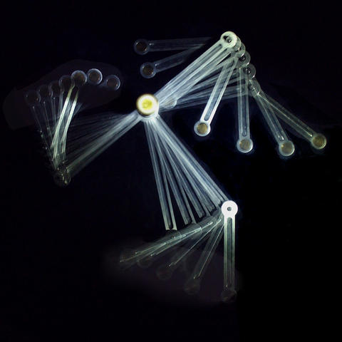
But this chaotic pendulum is different. It is an elegant work by San Francisco Bay area environmental artist and sculptor Ned Kahn. This is a quadruple pendulum, where a T-shaped bar pivots at the juncture, and three regular pendulums pivot off from its endpoints. The whole thing is encased in an acrylic frame so nobody gets their fingers stuck or heads bonked. And a knob lets the visitor crank the main T-shaped bar.

This simple structure is capable of some remarkable movements. A dance of sorts. Expressing a palette of behaviors.

I thought it would be interesting to simulate Kahn Quadruple Chaotic Pendulum in JavaScript. Please enjoy!

The Simulation

Use the mouse to give it a spin...

(This is a first pass; I'll improve things later. No, I have not compared the dimensions, masses, and time constants of this with the real pendulum. If you'd like to look at the code, it's here. About 6 pages.)

Why is the movement of this device so fascinating?

Normally mechanical devices operate on individual axes. Like on a robot; each servo motor has the responsibility of positioning a particular piece to an intended angle, and it goes about doing that job, meeting that spec, and applying power to get that peice to that angle.

Here there are no servo motors. Instead energy is being transferred between potential energy and kinetic energy, with the total kinetic + potential energy remaining constant. The potential energy is due to the height of the masses. The kinetic energy is due to the speed of the masses.

It turns out that this is very similar to the way human and mobile animals move around. We naturally minimize the energy we use to get a particular task done. And robots typically don't do that.

Derivation

The system is described with four angles, the angular position of the T Bar and the three small pendulums. And the derivatives of those. We'll number them; 0 is the T Bar on top, and 1, 2, and 3 are the smaller pendulums, left to right.

We'll be using the Lagrange approach; calculating the kinetic and potential energies of the system, and finding the accelerations. This is pretty straightforward, but the math is error-prone as all hell, so I'm writing it out here to keep things straight.

Here are the x,y positions of the endpoints of the T Bar:

\begin{aligned} (x, y)_{l e f t} & = (- l_{0} \cos θ_{0}, - l_{0} \sin θ_{0}) \\ (x, y)_{b o t t o m} & = (l_{0} \sin θ_{0}, - l_{0} \cos θ_{0}) \\ (x, y)_{r i g h t} & = (l_{0} \cos θ_{0}, l_{0} \sin θ_{0}) \end{aligned}

Calculate the kinetic energy, T, and the potential energy, V, (those are traditional Lagrange variable names) of all four parts, and add them up.

T = T_{0} + T_{1} + T_{2} + T_{3}

T_{i} = \frac{1}{2} m_{i} v_{i}^{2}

V = V_{0} + V_{1} + V_{2} + V_{3}

V_{i} = - g m_{i} y_{i}

\begin{aligned} T_{0} & = \frac{1}{2} m_{0} l_{0}^{2} \dot{θ_{0}^{2}} \\ V_{0} & = - g m_{0} l_{0} \cos θ_{0} \\ T_{1} & = \frac{1}{2} m_{1} (l_{0}^{2} \dot{θ_{0}^{2}} + l_{1}^{2} \dot{θ_{1}^{2}} + 2 l_{0} l_{1} {\dot{θ}}_{0} {\dot{θ}}_{1} \sin (θ_{0} - θ_{1})) \\ V_{1} & = - g m_{1} (l_{0} \sin θ_{0} + l_{1} \cos θ_{1}) \\ T_{2} & = \frac{1}{2} m_{2} (l_{0}^{2} \dot{θ_{0}^{2}} + l_{2}^{2} \dot{θ_{2}^{2}} + 2 l_{0} l_{2} {\dot{θ}}_{0} {\dot{θ}}_{2} \cos (θ_{0} - θ_{2})) \\ V_{2} & = - g m_{2} (l_{0} \cos θ_{0} + l_{2} \cos θ_{2}) \\ T_{3} & = \frac{1}{2} m_{3} (l_{0}^{2} \dot{θ_{0}^{2}} + l_{3}^{2} \dot{θ_{3}^{2}} - 2 l_{0} l_{3} {\dot{θ}}_{0} {\dot{θ}}_{3} \sin (θ_{0} - θ_{3})) \\ V_{3} & = - g m_{3} (- l_{0} \sin θ_{0} + l_{3} \cos θ_{3}) \end{aligned}

Find the total kinetic energy, T:

\begin{aligned} T = & \frac{1}{2} (m_{0} + m_{1} + m_{2} + m_{3}) l_{0}^{2} \dot{θ_{0}^{2}} \\ + \frac{1}{2} m_{1} l_{1}^{2} \dot{θ_{1}^{2}} + m_{1} l_{0} l_{1} {\dot{θ}}_{0} {\dot{θ}}_{1} \sin (θ_{0} - θ_{1}) \\ + \frac{1}{2} m_{2} l_{2}^{2} \dot{θ_{2}^{2}} + m_{2} l_{0} l_{2} {\dot{θ}}_{0} {\dot{θ}}_{2} \cos (θ_{0} - θ_{2}) \\ + \frac{1}{2} m_{3} l_{3}^{2} \dot{θ_{3}^{2}} - m_{3} l_{0} l_{3} {\dot{θ}}_{0} {\dot{θ}}_{3} \sin (θ_{0} - θ_{3}) \end{aligned}

Find the total potential energy, V:

\begin{aligned} V = & - g (l_{0} (m_{0} + m_{2}) \cos θ_{0} + l_{0} (m_{1} - m_{3}) \sin θ_{0} + m_{1} l_{1} \cos θ_{1} + m_{2} l_{2} \cos θ_{2} + m_{3} l_{3} \cos θ_{3}) \end{aligned}

Calculate the Lagrange:

L = T - V

\begin{aligned} L & = \frac{1}{2} (m_{0} + m_{1} + m_{2} + m_{3}) l_{0}^{2} \dot{θ_{0}^{2}} \\ + \frac{1}{2} m_{1} l_{1}^{2} \dot{θ_{1}^{2}} + m_{1} l_{0} l_{1} {\dot{θ}}_{0} {\dot{θ}}_{1} \sin (θ_{0} - θ_{1}) \\ + \frac{1}{2} m_{2} l_{2}^{2} \dot{θ_{2}^{2}} + m_{2} l_{0} l_{2} {\dot{θ}}_{0} {\dot{θ}}_{2} \cos (θ_{0} - θ_{2}) \\ + \frac{1}{2} m_{3} l_{3}^{2} \dot{θ_{3}^{2}} - m_{3} l_{0} l_{3} {\dot{θ}}_{0} {\dot{θ}}_{3} \sin (θ_{0} - θ_{3}) \\ + g (l_{0} (m_{0} + m_{2}) \cos θ_{0} + l_{0} (m_{1} - m_{3}) \sin θ_{0} + m_{1} l_{1} \cos θ_{1} + m_{2} l_{2} \cos θ_{2} + m_{3} l_{3} \cos θ_{3}) \end{aligned}

Find the partial derivatives of L over the angles:

\begin{aligned} \frac{\partial L}{\partial θ_{0}} = & m_{1} l_{0} l_{1} {\dot{θ}}_{0} {\dot{θ}}_{1} \cos (θ_{0} - θ_{1}) \\ - m_{2} l_{0} l_{2} {\dot{θ}}_{0} {\dot{θ}}_{2} \sin (θ_{0} - θ_{2}) \\ - m_{3} l_{0} l_{3} {\dot{θ}}_{0} {\dot{θ}}_{3} \cos (θ_{0} - θ_{3}) \\ - g l_{0} (m_{0} + m_{2}) \sin θ + g l_{0} (m 1 - m 3) \cos θ_{0} \\ \frac{\partial L}{\partial θ_{1}} = & - m_{1} l_{0} l_{1} {\dot{θ}}_{0} {\dot{θ}}_{1} \cos (θ_{0} - θ_{1}) - g m_{1} l_{1} \sin θ_{1} \\ \frac{\partial L}{\partial θ_{2}} = & m_{2} l_{0} l_{2} {\dot{θ}}_{0} {\dot{θ}}_{2} \sin (θ_{0} - θ_{2}) - g m_{2} l_{2} \sin θ_{2} \\ \frac{\partial L}{\partial θ_{3}} = & m_{3} l_{0} l_{3} {\dot{θ}}_{0} {\dot{θ}}_{3} \cos (θ_{0} - θ_{3}) - g m_{3} l_{3} \sin θ_{3} \end{aligned}

Find the partial derivatives of L over the angular velocities:

\begin{aligned} \frac{\partial L}{\partial {\dot{θ}}_{0}} = & (m_{0} + m_{1} + m_{2} + m_{3}) l_{0}^{2} {\dot{θ}}_{0} \\ + m_{1} l_{0} l_{1} {\dot{θ}}_{1} \sin (θ_{0} - θ_{1}) + m_{2} l_{0} l_{2} {\dot{θ}}_{2} \cos (θ_{0} - θ_{2}) - m_{3} l_{0} l_{3} {\dot{θ}}_{3} \sin (θ_{0} - θ_{3}) \\ \frac{\partial L}{\partial {\dot{θ}}_{1}} = & m_{1} l_{1}^{2} \dot{θ_{1}} + m_{1} l_{0} l_{1} \dot{θ_{0}} \sin (θ_{0} - θ_{1}) \\ \frac{\partial L}{\partial {\dot{θ}}_{2}} = & m_{2} l_{2}^{2} \dot{θ_{2}} + m_{2} l_{0} l_{2} \dot{θ_{0}} \cos (θ_{0} - θ_{2}) \\ \frac{\partial L}{\partial {\dot{θ}}_{3}} = & m_{3} l_{3}^{2} \dot{θ_{3}} - m_{3} l_{0} l_{3} \dot{θ_{0}} \sin (θ_{0} - θ_{3}) \end{aligned}

Now, take the time derivative of those:

\begin{aligned} \frac{d}{d t} (\frac{\partial L}{\partial {\dot{θ}}_{0}}) = & (m_{0} + m_{1} + m_{2} + m_{3}) l_{0}^{2} \ddot{θ_{0}} \\ + m_{1} l_{0} l_{1} {\ddot{θ}}_{1} \sin (θ_{0} - θ_{1}) + m_{1} l_{0} l_{1} ({\dot{θ}}_{0} - {\dot{θ}}_{1}) {\dot{θ}}_{1} \cos (θ_{0} - θ_{1}) \\ + m_{2} l_{0} l_{2} {\ddot{θ}}_{2} \cos (θ_{0} - θ_{2}) - m_{2} l_{0} l_{2} ({\dot{θ}}_{0} - {\dot{θ}}_{2}) {\dot{θ}}_{2} \sin (θ_{0} - θ_{2}) \\ - m_{3} l_{0} l_{3} {\ddot{θ}}_{3} \sin (θ_{0} - θ_{3}) - m_{3} l_{0} l_{3} ({\dot{θ}}_{0} - {\dot{θ}}_{3}) {\dot{θ}}_{3} \cos (θ_{0} - θ_{3}) \\ \frac{d}{d t} (\frac{\partial L}{\partial {\dot{θ}}_{1}}) = & m_{1} l_{1}^{2} \ddot{θ_{1}} + m_{1} l_{0} l_{1} {\ddot{θ}}_{0} \sin (θ_{0} - θ_{1}) + m_{1} l_{0} l_{1} {\dot{θ}}_{0} ({\dot{θ}}_{0} - {\dot{θ}}_{1}) \cos (θ_{0} - θ_{1}) \\ \frac{d}{d t} (\frac{\partial L}{\partial {\dot{θ}}_{2}}) = & m_{2} l_{2}^{2} \ddot{θ_{2}} + m_{2} l_{0} l_{2} {\ddot{θ}}_{0} \cos (θ_{0} - θ_{2}) - m_{2} l_{0} l_{2} {\dot{θ}}_{0} ({\dot{θ}}_{0} - {\dot{θ}}_{2}) \sin (θ_{0} - θ_{2}) \\ \frac{d}{d t} (\frac{\partial L}{\partial {\dot{θ}}_{3}}) = & m_{3} l_{3}^{2} \ddot{θ_{3}} - m_{3} l_{0} l_{3} {\ddot{θ}}_{0} \sin (θ_{0} - θ_{3}) - m_{3} l_{0} l_{3} {\dot{θ}}_{0} ({\dot{θ}}_{0} - {\dot{θ}}_{3}) \cos (θ_{0} - θ_{3}) \end{aligned}

Now, bring them together, with the double dotted angles on the left and everthing else on the right.

\frac{d}{d t} (\frac{\partial L}{\partial {\dot{θ}}_{i}}) = \frac{\partial L}{\partial θ_{i}}

\begin{matrix} (m_{0} + m_{1} + m_{2} + m_{3}) l_{0}^{2} \ddot{θ_{0}} + m_{1} l_{0} l_{1} \sin (θ_{0} - θ_{1}) {\ddot{θ}}_{1} + m_{2} l_{0} l_{2} \cos (θ_{0} - θ_{2}) {\ddot{θ}}_{2} - m_{3} l_{0} l_{3} \sin (θ_{0} - θ_{3}) {\ddot{θ}}_{3} = \\ - m_{1} l_{0} l_{1} ({\dot{θ}}_{0} - {\dot{θ}}_{1}) {\dot{θ}}_{1} \cos (θ_{0} - θ_{1}) + m_{2} l_{0} l_{2} ({\dot{θ}}_{0} - {\dot{θ}}_{2}) {\dot{θ}}_{2} \sin (θ_{0} - θ_{2}) + m_{3} l_{0} l_{3} ({\dot{θ}}_{0} - {\dot{θ}}_{3}) {\dot{θ}}_{3} \cos (θ_{0} - θ_{3}) \\ + m_{1} l_{0} l_{1} {\dot{θ}}_{0} {\dot{θ}}_{1} \cos (θ_{0} - θ_{1}) - m_{2} l_{0} l_{2} {\dot{θ}}_{0} {\dot{θ}}_{2} \sin (θ_{0} - θ_{2}) - m_{3} l_{0} l_{3} {\dot{θ}}_{0} {\dot{θ}}_{3} \cos (θ_{0} - θ_{3}) \\ - g l_{0} (m_{0} + m_{2}) \sin θ_{0} + g l_{0} (m 1 - m 3) \cos θ_{0} \end{matrix}

\begin{aligned} m_{1} l_{0} l_{1} \sin (θ_{0} - θ_{1}) {\ddot{θ}}_{0} + m_{1} l_{1}^{2} {\ddot{θ}}_{1} & = - m_{1} l_{0} l_{1} {\dot{θ}}_{0} ({\dot{θ}}_{0} - {\dot{θ}}_{1}) \cos (θ_{0} - θ_{1}) - m_{1} l_{0} l_{1} {\dot{θ}}_{0} {\dot{θ}}_{1} \cos (θ_{0} - θ_{1}) - g m_{1} l_{1} \sin θ_{1} \\ m_{2} l_{0} l_{2} \cos (θ_{0} - θ_{2}) {\ddot{θ}}_{0} + m_{2} l_{2}^{2} {\ddot{θ}}_{2} & = m_{2} l_{0} l_{2} {\dot{θ}}_{0} ({\dot{θ}}_{0} - {\dot{θ}}_{2}) \sin (θ_{0} - θ_{2}) + m_{2} l_{0} l_{2} {\dot{θ}}_{0} {\dot{θ}}_{2} \sin (θ_{0} - θ_{2}) - g m_{2} l_{2} \sin θ_{2} \\ - m_{3} l_{0} l_{3} \sin (θ_{0} - θ_{3}) {\ddot{θ}}_{0} + m_{3} l_{3}^{2} {\ddot{θ}}_{3} & = m_{3} l_{0} l_{3} {\dot{θ}}_{0} ({\dot{θ}}_{0} - {\dot{θ}}_{3}) \cos (θ_{0} - θ_{3}) + m_{3} l_{0} l_{3} {\dot{θ}}_{0} {\dot{θ}}_{3} \cos (θ_{0} - θ_{3}) - g m_{3} l_{3} \sin θ_{3} \end{aligned}

Simplify

\begin{matrix} (m_{0} + m_{1} + m_{2} + m_{3}) l_{0}^{2} \ddot{θ_{0}} + m_{1} l_{0} l_{1} \sin (θ_{0} - θ_{1}) {\ddot{θ}}_{1} + m_{2} l_{0} l_{2} \cos (θ_{0} - θ_{2}) {\ddot{θ}}_{2} - m_{3} l_{0} l_{3} \sin (θ_{0} - θ_{3}) {\ddot{θ}}_{3} = \\ + m_{1} l_{0} l_{1} {\dot{θ}}_{1}^{2} \cos (θ_{0} - θ_{1}) - m_{2} l_{0} l_{2} {\dot{θ}}_{2}^{2} \sin (θ_{0} - θ_{2}) - m_{3} l_{0} l_{3} {\dot{θ}}_{3}^{2} \cos (θ_{0} - θ_{3}) \\ - g l_{0} (m_{0} + m_{2}) \sin θ_{0} + g l_{0} (m 1 - m 3) \cos θ_{0} \end{matrix}

\begin{aligned} m_{1} l_{0} l_{1} \sin (θ_{0} - θ_{1}) {\ddot{θ}}_{0} + m_{1} l_{1}^{2} {\ddot{θ}}_{1} & = - m_{1} l_{0} l_{1} {\dot{θ}}_{0}^{2} \cos (θ_{0} - θ_{1}) - g m_{1} l_{1} \sin θ_{1} \\ m_{2} l_{0} l_{2} \cos (θ_{0} - θ_{2}) {\ddot{θ}}_{0} + m_{2} l_{2}^{2} {\ddot{θ}}_{2} & = m_{2} l_{0} l_{2} {\dot{θ}}_{0}^{2} \sin (θ_{0} - θ_{2}) - g m_{2} l_{2} \sin θ_{2} \\ - m_{3} l_{0} l_{3} \sin (θ_{0} - θ_{3}) {\ddot{θ}}_{0} + m_{3} l_{3}^{2} {\ddot{θ}}_{3} & = m_{3} l_{0} l_{3} {\dot{θ}}_{0}^{2} \cos (θ_{0} - θ_{3}) - g m_{3} l_{3} \sin θ_{3} \end{aligned}

Simplify some more

\begin{matrix} (m_{0} + m_{1} + m_{2} + m_{3}) l_{0} \ddot{θ_{0}} + m_{1} l_{1} \sin (θ_{0} - θ_{1}) {\ddot{θ}}_{1} + m_{2} l_{2} \cos (θ_{0} - θ_{2}) {\ddot{θ}}_{2} - m_{3} l_{3} \sin (θ_{0} - θ_{3}) {\ddot{θ}}_{3} = \\ + m_{1} l_{1} {\dot{θ}}_{1}^{2} \cos (θ_{0} - θ_{1}) - m_{2} l_{2} {\dot{θ}}_{2}^{2} \sin (θ_{0} - θ_{2}) - m_{3} l_{3} {\dot{θ}}_{3}^{2} \cos (θ_{0} - θ_{3}) \\ - g (m_{0} + m_{2}) \sin θ_{0} + g (m 1 - m 3) \cos θ_{0} \end{matrix}

\begin{aligned} l_{0} \sin (θ_{0} - θ_{1}) {\ddot{θ}}_{0} + l_{1} {\ddot{θ}}_{1} & = - l_{0} {\dot{θ}}_{0}^{2} \cos (θ_{0} - θ_{1}) - g \sin θ_{1} \\ l_{0} \cos (θ_{0} - θ_{2}) {\ddot{θ}}_{0} + l_{2} {\ddot{θ}}_{2} & = l_{0} {\dot{θ}}_{0}^{2} \sin (θ_{0} - θ_{2}) - g \sin θ_{2} \\ - l_{0} \sin (θ_{0} - θ_{3}) {\ddot{θ}}_{0} + l_{3} {\ddot{θ}}_{3} & = l_{0} {\dot{θ}}_{0}^{2} \cos (θ_{0} - θ_{3}) - g \sin θ_{3} \end{aligned}

And from here we can use a little matrix math to solve for the four accelerations given the four positions and four velocities.