Harmonic Distortion, Odd- and Even-Order
J. Donald Tillman
Sept 2022
This article is a guided tour through the characteristics of Harmonic Distortion. Welcome.
In the audio world, there has been a lot of debate about odd and even order harmonic distortion; their qualities, timbre, audibility, and such. Sometimes boiling down to "even good, odd bad". But I thought the topic would be worth exploring a bit.
"Harmonic Distortion" has traditionally been a measure of the quality of an amplifier, or other audio device, with respect to its linearity. The ratio of the output voltage to the input voltage should be a constant value. And if you plot the output-vs-input on an XY plot you should see a perfectly straight line. And any curve, wiggle, or warp in that line would be a nonlinearity.
The procedure to measure harmonic distortion is to use the purest available source of a sine wave, apply it to the input, drive the unit at the intended level (often its rated output), and measure the output signal. Any nonlinearities in the unit would show up in the output as a misshapen sine wave, which would have additional harmonic content. So the harmonic distortion is the ratio of the level of the extraneous harmonic content to the sine wave.
For this article I created a triptych display that presents the curve, the wave, and the spectrum, all together, for various distortion curves. It's enlightening to see a mechanism from multiple angles simultaneously.
The Jupyter Notebook Python source code for the triptych displays is available here: https://github.com/dontillman/distortion-article.
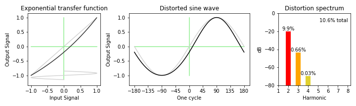
Exponential Curve
We'll start with an exponential curve. While ex is a very specific curve, it also serves as an example of the general case where the slope increases at higher x values.
The exponential curve is also very significant in electronics; the transfer function of a bipolar transistor is an exponential curve. Specifically:
$$I_E = I_{ES}({e^{V_{BE} / V_T} - 1)}$$Here are the curve, the distorted sine wave, and the harmonic distortion components:
For these graphs, the source is a +/- 1.0 Volt peak-to-peak sine wave. The left plot shows the nonlinear curve with the input on the X axis and the output on the Y axis. I placed a sideways sine wave at the bottom of the plot to help make that clear. The nonlinearity is scaled and biased to cover the same +/- 1.0 volt range as the input.
The middle plot shows the resulting distorted sine wave, and compares it to a proper sine wave.
The right plot shows the resulting spectral components of the distortion. To minimize distractions, the DC component and the fundamental have been removed, as well as any harmonics less than -80dB down. The harmonic colors are assigned from the Electronic Color Code so my electrical engineering readers will feel at home.
The distortion level and harmonic content varies with signal level. For demo purposes, the examples in this article the signal level have been hand-tweaked to generate a level of about 10% harmonic distortion. That's a lot in the hifi world, but smaller levels would be difficult to see.
Of course this is all in an abstract theoretical world, and in the real world things are a lot more complex.
So in this example, we see that an exponential nonlinearity creates multiple harmonics, both odd and even, but the 2nd harmonic predominates. Technically, an exponential distortion curve creates all harmonics, but they drop off pretty quickly.
The Parabolic Curve
The next curve is a parabola, or x2, curve.
For the parabola, and any other xn curves, we have to bias the signal up from zero center, else there would be all harmonics and no fundamental. So the approach is to bias the curve to the point where have 10% harmonic distortion. In this case, up 2.5 Volts.
The parabolic curve is also important because, due to their construction, Field Effect Transistors exhibit a square law transfer curve:
$$I_{DS} = I_{DSS} (1 - V_{GS} / V_P)^2$$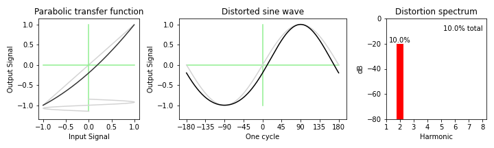
The parabolic curve is unique and especially interesting as its only distortion product is the second harmonic.
And this is consistent with the trigonometric identity:
$$\cos^2 \theta = {{\cos 2 \theta + 1} \over 2}$$There will be more on the parabolic curve later...
Other xn Curves
How about a cubic curve? Or a quartic, or x4, curve.
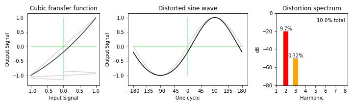
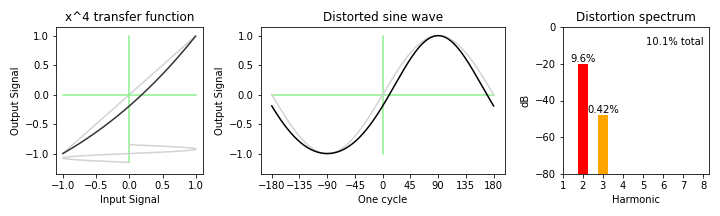
They're both remarkably similar, both in the shape of the curve and the harmonic content. And I think this is mostly due to the constraint of driving the stage to a 10% distortion level.
x3/2 Curve
Venturing on the other side of the parabola (ahem...), here is an x3/2 curve.
I am including this because because Marshall Leach's SPICE model of a vacuum tube uses an x3/2 curve:
$$i_P = K (\mu v_{GK} + v_{PK})^{3/2}$$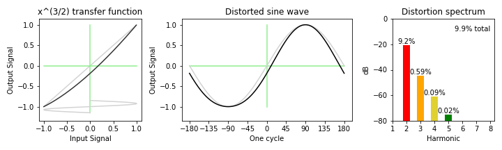
Symmetrical Mechanisms with Only Odd Harmonics
We say that a given nonlinearity is symmetrical when the curve for the negative half of the signal is the exact mirror-image opposite of the curve on positive half. For these situations, all the even harmonics cancel out and we are left with just odd harmonics.
This is a hyperbolic tangent, or tanh(), curve, which is mirror-image symmetrical.
The tanh() curve is also the large signal transfer function of a bipolar transistor pair differential amp circuit. So we see this used all over the place.
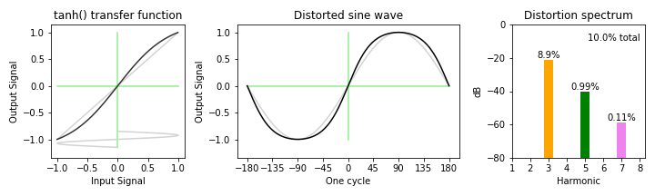
Sure enough, odd harmonics only.
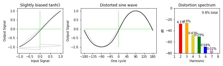
Turning Odd Harmonics into Even Harmonics
While a distortion of only odd harmonics is specific to a symmetrical mechanism, and has a readily identifiable spectral characteristic, it's incredibly easy to circumvent. All you have to do to convert a symmetrical curve to a non-symmetrical curve is to add a little bias voltage.
So here we take the tanh() curve above and bias the zero point down 0.15 Volts. The original 10% predominantly 2nd order harmonic distortion spreads out over seven harmonics, while keeping the total distortion about the same. That's a pretty dramatic result for such a simple change.
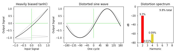
We can take it even further. If we bias the tanh() curve down significantly we can turn it into something very closely resembling a parobolic curve, with pretty much entirely 2nd harmonic distortion.
Eliminating Even Harmonics: Push-Pull
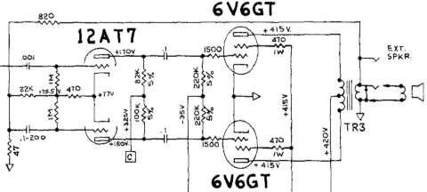
You can eliminate even harmonics by placing two stages in a push-pull arrangement.
Push-pull is the circuit topology used in almost every vacuum tube power amplifier. The signal goes through a "phase splitter" stage that delivers balanced positive and negative versions of the audio signal, and each of those drives an output stage on alternate ends of an output transformer. This topology naturally creates a symmetrical transfer function by cancelling the even-order harmonic distortion components.
For example, here is the schematic for the power amp on the classic Fender Deluxe guitar amp:
From a signal chain point of view, the result is effectively combining the original and inverted transfer functions.
$$f_{pushpull}(x) = f(x) - f(-x)$$If we have two devices with the vacuum tube x3/2 curve above and place them in a push-pull arrangement, the result is the original curve with the even harmonics removed.
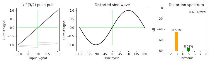
And since the 2nd harmonic was by far the most prominent, the result is a total distortion level reduced by well over an order of magnitude. And this is the first plot with no visible distortion on the sine wave.
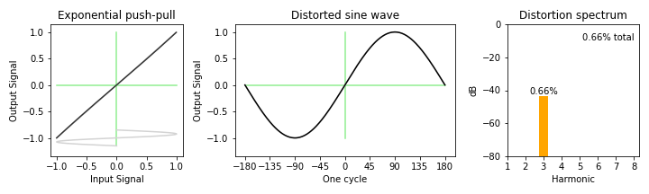
The effect on a bipolar transistor exponential curve is almost identical. Suggesting that, based only on theoritical curves, that vacuum tube and bipolar transistor output stages are nearly identical. Of course in real life things are more complicated.
A push-pull version of the parabolic distortion curve is a special case; all of the distortion is in the second harmonic, and it mathematically cancels completely:
$$(2.5 + x)^2 - (2.5 - x)^2 = (6.25 + 5x +x^2) - (6.25 - 5x + x^2) = 10x$$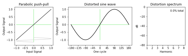
You can also do a push-pull arrangement with the tanh() stage above that was heavily biased to be predominantly 2nd harmonic distortion and the result is the same. But it would be an example of a symmetrical odd-harmonic stage, biased to be even harmonics, and then used in a push-pull pair to be odd harmonics again. It seems like a pointless excersize at first... but maybe not.
Two Stages in a Row
Discussions of harmonic distortion and devices generally assume that there's only one device. Near zero pieces of audio equipment have exactly one stage. Usually there are multiple stages, in all kinds of configurations, parallel, series, whatever.
A single parabolic stage has only 2nd harmonic distortion. But what happens if we put the signal through two parabolic stages in series? 4th harmonic?
(For these plots, the signal is adjusted for unity gain and zero offset between the two stages.)
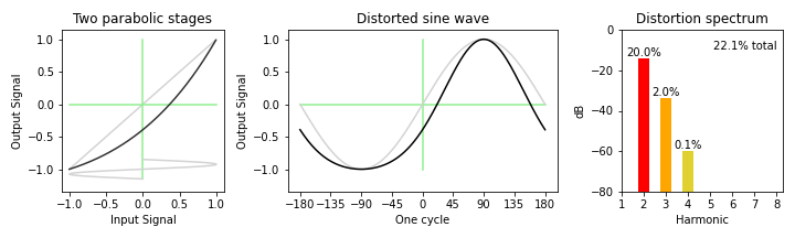
Interesting; the 2nd harmonic distortion literally doubled, which makes some sense. And the 3rd and 4th harmonics were added as a side effect.
However... that probably won't happen in practical circuits. If I have a gain stage, whether it is a vacuum tube, bipolar transistor, or FET, that gain stage will most likely be wired up to invert the signal ("common cathod", "common emitter", "common source").
For example, here is the preamp of the aforementioned Fender Deluxe:
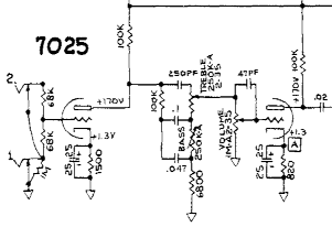
The input goes through the first vacuum tube gain stage, with a gain of 50 or so, and inverted in the process, and then the signal gets knocked down by the passive tone controls, and the volume control, to roughly the original strength, depending on the settings, and gets another boost, and another inversion, by the second "recovery" stage.
Here is the same curve as above, but with an inversion in between the two stages.
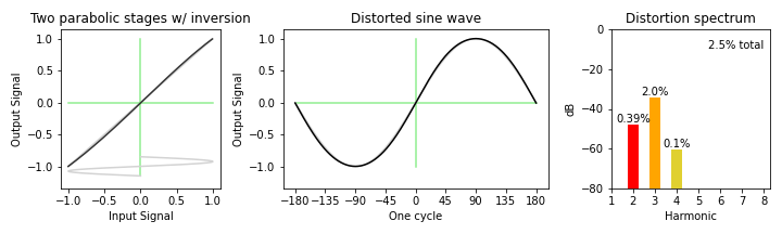
We went from 22% distortion down to 2.5% just by inverting an audio signal? What happened?
The 2nd harmonic distortion component in the second stage is of the opposite polarity to the 2nd harmonic distortion of first stage, and mostly cancelled it.
I think it's delightful how an "organic" distortion cancelling mechanism is built in to the regular design of vacuum tube preamps, and it goes by unnoticed.
And yes, one of my analog design techniques is to set things up so that the nonlinearities of adjacent stages cancel.
Local Feedback
Finally, we can add negative feedback. Here I'm referring to small amounts of local feedback, such as an emitter resistor. Opamp circuits involve large amounts of global feedback, and they work very differently, more like a servo than an amplifier. And that's another topic entirely.
Local feedback has several effects; it reduces harmonic distortion overall, it changes the spectrum of the distortion, it reduces the output level, and it reduces the level of the signal coming in to the nonlinear transfer function, which reduces the distortion some more.
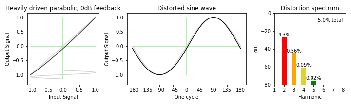
Just as an example, here is the parabolic curve, normally 10% 2nd harmonic distortion only, but with 6dB feedback (a loop gain of 1).
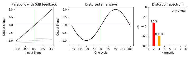
Given the reduced input signal level, you have the opportunity to drive the signal harder to cause a given level of distortion. So things could get a little confusing at that point. You'd really need to do a proper analysis of your specific circuit. In this case, the harmonics look nothing like the original situation.
Summary
'Hope you enjoyed the tour. Overall, it seems to me that the odd/even classification of harmonic distortion is one of those cases where if all you've got is a hammer then everything looks like a nail. Yes, odd and even order distortion is eminently classifiable. But it's also quite malliable, depending on the circuit context.
References
- Jupyter Notebook Python source code for the triptych displays https://github.com/dontillman/distortion-article.
- SPICE Models for Vacuum Tube Amplifiers, W. Marshall Leach, Jr., Journal of the Audio Engineering Society, Vol. 33, No. 3, March 1995
- Bipolar Transistor Wikipedia
- Junction Field Effect Transistor Wikipedia